March 2024 – A Point of View.

Romanian Master of Mathematics, 2024. NT problems!

Two nice number theory (NT) flavored problems were given at the recent RMM (Romanian Master of Mathematics) competition. The only needed knowledge of NT that one has to have in order to solve them consists of the following two facts. For any prime $p,$ 1) If $n_i\not\equiv 0\pmod p, i=1,2$ then $n_1n_2\not\equiv 0\pmod p.$ 2) For any integers $r,n_1,n_2$ with $n_1\not\equiv n_2\pmod p$ we have $n_1+r\not\equiv 0\pmod p$ or $n_2+r\not\equiv 0\pmod p.$
Yes, a fifth grader knows it. Still the problems are not so easy. Some people want strict boundaries between different subjects in math competitions. They want for example some “pure” NT problems. Of course, mathematics has different subjects. But they share common methods and technique called Math. Take for example the Euler’s theorem about the totient function.

$\displaystyle a^{\varphi(n)}\equiv 1\pmod n\text{ if } (a,n)=1\qquad(1).$

The proof of it goes like that. One takes the set $A$ of all residues $\{r_1,r_2,\dots,r_m\}$ modulo $n$ that are coprime with $n$ . Then one takes $a\in A$ and considers the set $A':=\{ar_1,ar_2,\dots,ar_m\}.$ It follows from very basic facts that all these numbers give distinct residues modulo $p$ and all of them are coprime with $n.$ This allows us to conclude $A=A'$ , that is, the second system of residues is just a permutation of the first one. Multiplying the elements in $A$ and the elements in $A'$ (the same sets modulo $p$ ), we get

$\displaystyle a^m\cdot r_1r_2\cdots r_m\equiv r_1r_2\cdots r_m\pmod p.$

Since $m=\varphi(n)$ (by the definition of $\varphi$ ), the result in $(1)$ follows.
One might argue that there is very little NT stuff in this proof – you take a set, multiply each of its elements and get a permutation – this could be seen as combinatorics! But it is still a number theory theorem. I thinks it’s silly to argue whether a problem is combinatorics or number theory, or something else. They all intertwine.
Let’s continue with the two mentioned NT problems from RMM 2024.

RMM 2024, Problem 2. Consider an odd prime $p$ and a positive integer $N < 50p$ . Let $a_1, a_2, \ldots , a_N$ be a list of positive integers less than $p$ such that any specific value occurs at most $\frac{51}{100}N$ times and $a_1+a_2 + \cdots + a_N$ is not divisible by $p$ . Prove that there exists a permutation $b_1, b_2, \ldots , b_N$ of the $a_i$ such that, for all $k = 1, 2, \ldots , N$ , the sum $b_1 + b_2 + \cdots + b_k$ is not divisible by $p$ .
(Will Steinberg, United Kingdom)

The following solution is similar to the official one, but it emphasizes on a constructive algorithm. Suppose we initially have a multiset $A$ of residues modulo $p$ (we allow $0\in A$ ) that satisfies the condition

$\displaystyle \text{Each value in }A\text{ occurs at most } \left\lceil \frac{|A|}{2}\right\rceil \text{ times.}\qquad(1)$

Then $A$ can be arranged in a row $b_1,b_2,\dots,b_N, N:=|A|$ that satisfies the problem’s condition. This arrangement can be done via a greedy algorithm with a little bit common sense. Here it is.
Because of condition $(1)$ there are at least two distinct values in $A$ . So, we start putting the elements of $A$ in a row, each time picking a residue that avoids a certain residue, i.e. it avoids the sum of the already arranged residues taken with a negative sign. Assume at some moment, we have a multiset $A'$ such that some of its values, say $r$ occurs exactly $\left\lceil {|A'|}/{2}\right\rceil$ times. We try to pick this value, and if we cannot do this, because we would hit $0$ , then we pick another residue $r_1\neq r$ , put it in the row and we put $r$ immediately after $r_1$ . Thus, we comply with the given condition and we are at position with a multiset $A''$ that consists of $|A'|-2$ elements. The point is that $A''$ still satisfies $(1)$, so we can continue with the same algorithm.

It remains to see what to do when initially some value $r$ in $A$ occurs $k$ times and $k>\left\lceil {|A|}/{2}\right\rceil$ times. This time we want $0\notin A$ . So,

$\displaystyle \left\lceil {|A|}/{2}\right\rceil < k<\frac{51}{100}|A|\qquad (2).$

Now, we put all the elements equal to $r$ , but no more than $p-1$ of them, one after another in a row. Any partial sum of this row is not $0$ , since $0\notin A$ . Because of $(2)$ and the fact that $|A|<50p$ , it easily follows that the remaining elements form a multiset $A'$ that satisfies $(1)$ . Further, we proceed with the above algorithm, avoiding a certain residue each time. $\square$

The next problem is problem 4 from the same competition.

RMM 2024, problem 4. Fix integers $a$ and $b$ greater than $1$ . For any positive integer $n$ , let $r_n$ be the (non-negative) remainder that $b^n$ leaves upon division by $a^n$ . Assume there exists a positive integer $N$ such that $\displaystyle r_n < \frac{2^n}{n}$ for all integers $n\geq N$ . Prove that $a$ divides $b$ .
(Pouria Mahmoudkhan Shirazi, Iran)

Assume that $b$ is not multiple of $a.$ Hence, $\displaystyle \frac{b}{a}=\frac{p}{q}$ where $(p,q)=1$ and $q>1$ . In this case we’ll prove something stronger. Namely, it’s even not possible that $r_n<\varepsilon_n a^n$ , where $\displaystyle \lim_{n\to \infty}\varepsilon_n =0$ , that is, it’s not possible that $r_n=o(a^n)$ .

Assume on the contrary it holds. Thus,

$\displaystyle b^n=ka^n+\varepsilon_n a^n.$

Multiplying both sides by $b$ it yields

$\displaystyle b^{n+1}=k\frac{b}{a}a^{n+1}+\varepsilon_n \frac{b}{a}a^{n+1}.$

It means that

$\displaystyle \varepsilon_{n+1}=\left\{k\frac{p}{q}+\varepsilon_n \frac{p}{q} \right\}$

where $\{\cdot\}$ denotes the fractional part. Now, for sufficiently large $n$ we have $\displaystyle \varepsilon_n \frac{p}{q}<\frac{1}{q},$ since $\displaystyle \varepsilon_n\to 0$ . Note that $\displaystyle k\frac{p}{q}$ is either integer or its distance to the nearest integer is at least $1/q.$ It gives us $\displaystyle \varepsilon_{n+1}>\varepsilon_n.$ This leads us to contradiction if we take a special $\displaystyle \varepsilon_n$ such that $\displaystyle \varepsilon_i<\varepsilon_n, \forall i>n.$ It is possible since $\varepsilon_n\to 0.$ $\square$

This problem is similar to Izho 2021, problem 1 – see [3] – the idea is the same. In fact, we proved that for given positive integers $b>a$ and $b$ is not multiple of $a,$ we can find infinitely many $n$ such that the residue that $b^n$ leaves upon division by $a^n$ is greater than $Ca^n$ for some constant $C$ that depends only on $a$ and $b.$

References.
[1] RMM 2024, p.2 – AoPS thread.
[2] RMM 2024, p.4 – AoPS thread.
[3] IZhO 2021, p.1 – AoPS thread.

Almost All Binary Polynomials are Square Free. RMM 2024, Problem 6.

Here we consider problem 6 of the recent Romanian Master of Mathematics competition – a very difficult problem. Nobody solved it during the tournament. Let me point out a very similar problem – RMM Shortlist 2020, A1 – see [3], proposed by the same author. I think it’s of similar difficulty. In my opinion both are not suitable for a high school Olympiad level, although I like them because it’s real math. Maybe they fit for Miklos Schweitzer competition, but on the other hand both problems are known results – the current one by Filaseta and Konyagin – see [2] – so the papers can easily be found by searching the web.

Problem (RMM 2024, problem 6). A polynomial $P$ with integer coefficients is square-free if it is not expressible in the form $P = Q^2R$ , where $Q$ and $R$ are polynomials with integer coefficients and $Q$ is not constant. For a positive integer $n$ , let $P_n$ be the set of polynomials of the form

$\displaystyle 1 + a_1x + a_2x^2 + \cdots + a_nx^n\text{ with } a_1,a_2,\ldots, a_n \in \{0,1\}.$

Prove that there exists an integer $N$ such that for all integers $n \geq N$ , more than $99\%$ of the polynomials in $P_n$ are square-free.
(Navid Safaei, Iran)

The proof is based on the ideas I saw in [4] and consists of 3 main statements. The proof of the last one is a version of a problem we did in a blogpost here – see [1].

It boils down to prove that if we take a random polynomial in $P_n,$ the probability that it is not square-free tends to $0$ as $n\to \infty.$ Hereafter, we refer to polynomials in $P_n$ that are not square-free as bad polynomials, and to the square-free ones as good. So, in other words, if we take a random polynomial in $P_n,$ the probability that it is bad tends to $0$ as $n\to \infty.$ Here are the milestones of our plan.

Claim 1. We’ll show that if we fix a natural number $d,$ the probability of taking a bad polynomial $P$ in $P_n$ with $P=Q^2R$ and $\deg(Q)\ge d$ can be made as small as we want if $d$ is large enough.
Claim 2. We prove that there are finitely many $Q$ with integer coefficients and $\deg(Q)<d$ for which there exists $n$ and $P\in P_n$ such that $Q\mid P.$
Claim 3. We prove that for each fixed polynomial with integer coefficients $Q,$ the probability of taking a polynomial $P\in P_n$ so that $Q\mid P$ tends to $0$ as $n\to \infty.$

Suppose that we already have the above three claims proven. The second claim ensures that there are only finitely many integer polynomials $Q_1,Q_2,\dots,Q_m$ with degrees less than $d$ that can divide a binary polynomial $P$ .
For any fixed $n$ we take a random polynomial $P\in P_n$ and let us introduce the following events. Hereafter, $Q$ denotes a polynomial with integer coefficients.

$\displaystyle E_1:= (P \text{ is bad and there exists }Q, \deg(Q)\ge d, \text{ such that }Q^2\mid P)$

$\displaystyle E_2:= (P \text{ is bad and if } Q^2\mid P \text{ then }\deg(Q)< d)$

$\displaystyle E_2':=(\text{there exists } i\,,\,1\le i\le m \text{ such that }Q_i\text{ divides } P)$

$\displaystyle E_2'(i):= (Q_i\text{ divides } P)$

Apparently,

$\displaystyle E_2\subset E_2'\subset \bigcup_{i=1}^m E_2'(i)$

which implies

$\displaystyle \mathbb{P}(E_2)\le \sum_{i=1}^m \mathbb{P}(E_2'(i)).$

Fix some $\varepsilon>0.$ The first claim shows that we can choose sufficiently large $d$ such that for any $n\ge d$ we have $\mathbb{P}(E_1)<\varepsilon.$ According to the third claim, we can choose $N_i$ such that for $n\ge N_i$ we have $\mathbb{P}(E_2'(i))<\varepsilon/m.$ Therefore, for $n>\max\{d,N_i: 1\le d\le m\}$ we have

$\displaystyle \mathbb{P}(P\text{ is bad })\le \mathbb{P}(E_1)+ \sum_{i=1}^m \mathbb{P}(E_2'(i))\le 2\varepsilon.$

This means that the probability of taking a bad polynomial can be made as small as we want by choosing a sufficiently large $n.$ It remains to prove the three statements.

Proof of Claim 1. Dealing with large squares dividing binary polynomials.

Let $d$ be a natural number. Hereafter, $Q$ and $R$ denote polynomial with integer coefficients and $P$ is a binary polynomial of degree $n.$ Suppose $P=Q^2R$ where $\deg(Q)=s\ge d.$ We reduce the polynomials $P,Q,R$ modulo 2, i.e. we substitute each coefficient with its residue modulo 2, thus obtaining new polynomials $P,\overline{Q}, \overline{R}$ ( $P$ remains the same). Clearly

$\displaystyle P=\left(\overline{Q}\right)^2\overline{R}\qquad(1).$

We can assume that $Q$ is a monic polynomial, hence $\deg\left(\overline{Q}\right)=\deg(Q)=s.$ Clearly, $\deg(\overline{R})=n-2s.$ Since $\overline{Q}$ has $s+1$ binary coefficients and $\overline{R}$ has $n-2s+1$ ones, all possible options for them are $2^{s+1}\cdot 2^{n-2s+1}=2^{n-2s+2}.$ Thus, the number of polynomials $P$ that satisfies $(1)$ is at most $2^{n-2s+2}.$ Therefore,

$\displaystyle \mathbb{P}(P=Q^2R, \deg{Q}=s)\le \frac{2^{n-2s+2}}{2^n}=4\cdot 2^{-s} .$

This yields,

$\displaystyle \mathbb{P}(E_1)\le 4\sum_{s\ge d}2^{-s}=\frac{1}{2^{d-3}}.$

which proves Claim 1.

Proof of Claim 2. Only finitely many “small” polynomials can divide a binary polynomial.

Let $P$ be a binary polynomial of degree $n.$ First to see that all roots of $P$ lie in the disk $\{z\in\mathbb{C} : |z|<2\}.$ Assume on the contrary $P(z)=0$ and $|z|\ge 2.$ Then

$\displaystyle |z|^n=|a_nz^n|=\left|\sum_{i=0}^{n-1}a_iz^i \right|\le \sum_{i=0}^{n-1}|a_iz^i|$

$\displaystyle \le \sum_{i=0}^{n-1}|z|^i=\frac{|z|^n-1}{|z|-1}<|z|^n,$

contradiction. Suppose now $Q\mid P\,,\, \deg(Q)=s\le d$ and the senior coefficient of $Q$ is $1.$ Let $z_1,z_2,\dots,z_s$ are the roots of $Q$ . The magnitude of all of them is less than $2.$ Using the Vieta formulas, we see that the coefficients of $Q$ are less than some expression that depends only on $d.$ Since these coefficients are integers, the options for $Q$ are finitely many, they are bounded by some constant that depends only on $d,$ but not on $n.$

Proof of Claim 3. The probability that a binary polynomial is a multiple of a fixed polynomial is small.

Let $Q$ be a fixed polynomial of integer coefficients and suppose $Q\mid P, P\in P_n.$ Let $\xi$ be a root of $Q.$ It follows $P(\xi)=0.$ Note that $\xi\neq 0,$ that’s why $a_0=1$ in the definition of $P_n.$ Take the set $S={xi^i: i=1,2,\dots,n}$ . Let us first consider the case when $|S|=n$ , i.e. $\xi$ is not a root of unity. The equality

$\displaystyle -1=\sum_{i=1}^{n} a_i\xi^i, a_i\in\{0,1\}$

just means that the sum of elements of some subset of $S$ is $-1$

Lemma 1. Let $S$ be a set of $n$ distinct complex numbers and $r\in\mathbb{C}.$ The probability that the sum of the elements of a random subset of $S$ is $r$ is less than $\displaystyle \frac{2}{n+1}$ .

Proof. I considered and proved this claim in a blog post, see [1]. Call a subset of $S$ bad if the sum of its elements is $r.$ As usual, a subset of $S$ can be represented as a binary vector $\{0,1\}^n$ each bit indicates if an element is in the set or not. The idea is simple. For any binary vector $b$ that corresponds to a bad subset we consider the unit sphere (by Hamming distance) centered at $b$ , that is, the set of all binary vectors that differ from $b$ at exactly one bit. Their number is $n.$ Non of them is a bad binary vector. That is, each bad binary vector is surrounded by $n$ good ones. A bit care is needed to ensure that the unit spheres corresponding to distinct bad vectors do not intersect – see in [1]. So, the estimate follows. $\square$

Claim 3 follows from Lemma 1 if $|S|=n.$ It remains to consider the case when $S$ is a multiset. Note that $0\notin S$ since $\xi\neq 0.$ Let $k$ be he the smallest number with $\xi^k=1$ . We have a multiset $S$ with $k$ groups, each one consists of (almost) $n/k$ equal values. If $k$ is large (e.g. $k>\sqrt{n}$ ), we can do the same trick as in Lemma 1 (flipping the bit of the first element of each group – we can number them) and obtain that the probability of taking a bad binary vector is less than $\displaystyle \frac{2}{k+1}\le \frac{2}{\sqrt n}$ .

In case $k$ is small ( $k<\sqrt n$ ), we take the group $G$ with the largest number of elements, say $m, m\ge n/k$ . Take a bad binary vector $b$ and let the number of chosen elements that are in $G$ is $s$ . Since all the elements in $G$ are the same (they have the same value), every binary vector with the same bits as $b$ outside $G$ , and such that the number of 1’s bits corresponding to the elements of $G$ is different from $s$ is not bad. So, the portion of the bad vectors for any fixed binary values corresponding to elements outside $G$ is at most

$\displaystyle \frac{\binom{m}{s}}{2^{m}} \le \frac{C}{\sqrt m}$ .

where $C$ is a constant. Therefore, the probability of taking a bad binary vector is less than $\displaystyle \frac{C}{\sqrt m}\le \frac{C}{\sqrt[4]{n}}$

This means that for a fixed polynomial $Q$ , the probability of randomly taken $P\in P_n$ is multiple of $Q$ is $O(n^{-1/4}),$ so it tends to zero as $n\to\infty.$

Comment

This solution has several crucial moments. The most difficult part (in my opinion) is to see that the probability of a binary polynomial $P$ be multiple of $Q^2$ where $Q$ is an integer polynomial of some large degree, is small (it’s $o(1)$ ). It involves a reduction modulo $2$ . The second part is to see that there are only finitely many polynomials with small degrees that can divide some binary polynomial $P.$ To see this we bound their coefficients. This is not hard to see, but it’s meaningful only if you got the first idea. In the third place comes the idea that for any fixed $Q$ , the portion of the binary polynomials multiple of $Q$ tends to $0$ as $n\to \infty$ . I would say that it’s doable in real time, but only if you get to that point.

References.
[1] Hamming distance in Olympiad problems. Part 2.
[2] Squarefree values of polynomials all of whose coefficients are 0 and 1, M. Filaseta, S. Konyagin, Acta Arith., 74(3): 191-205, 1996
[3] A polynomial with coefficients +/-1 very likely to be irreducible. RMM 2020 Shortlist.
[4] AoPS thread on this problem

A Special Discrete Harmonic Function. Part 2.

This is a continuation of the previous post – see [1]. I’ll show a more elegant way that will allow us to find all solutions to the functional equation we considered, but it requires a tool called the Krein – Milman theorem. The outline of this post is to first recall the problem, then Krein – Milman theorem and the intuitive motivation behind it. We will finally apply it.

Problem (China MO). Let $\displaystyle f:\mathbb{Z}_{\ge 0}\times \mathbb{Z}_{\ge 0}\to \mathbb{R}_{\ge 0}$ be a function satisfying

$\displaystyle f(x,y)=f(x+1,y)+f(x,y+1)\,;\, f(0,0)=1$

Prove that

$\displaystyle \big(f(x,0)\big)^2\le f(2x,0), \forall x\in\mathbb{Z}{\ge 0}.$

In the previous post – see [1] – we proved it using finite differences and making some estimates.

Krein – Milman Theorem.

Let $K$ be a convex set inside some real vector space $X$ . We say $x_0\in K$ is an extreme point (also called a corner point) of $K$ if it does not lie in the interior of any line segment between two points of $K$ . In figure 1 below, we have a convex quadrilateral $K=ABCD$ whose extreme points are the vertices $A,B,C,D$ (in red). All the other points of $K$ are not extreme points, because we can construct a segment lying in $K$ that contains in its interior any other point of $K$ except the red corners.

Roughly speaking, Krein-Milman theorem says that any convex set $K$ is the convex hull of its extreme points. Here is the precise statement.

Krein-Milman Theorem. Let $X$ be a locally convex topological vector space and $K\subset X$ is a compact convex set. Then $K$ is the closed convex hull of its extreme points.

So, the theorem is applicable when $X$ is some abstract space, say a space of certain functions. This theorem is intuitively “obvious” when $X$ is the two or three-dimensional Euclidean space (see figure 1). In this case the claim was proved by Minkowski (1911). It was then extended to the $n$ -dimensional space. When dealing with final dimensional vector spaces we do not need the word “closed “(convex hull) so then $K$ is simply the convex hull of its extreme points. In the general case, proved by Mark Krein and David Milman in 1940, it’s essential to take the closure of the convex hull. There are counterexamples showing a compact convex set such that the convex hull of its extreme points is not closed. We proceed with a proof of the original problem as an application of the Krein-Milman theorem.

A Solution.

Let us calibrate the function $f$ by setting $g(x,y):=2^{x+y}f(x,y)$ so that the new function satisfies

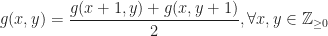
$\displaystyle g(x,y)=\frac{g(x+1,y)+g(x,y+1)}{2}, \forall x,y\in\mathbb{Z}_{\ge 0}$

$\displaystyle g(x,y)\ge 0, \forall x,y\in\mathbb{Z}_{\ge 0}\text{ and } g(0,0)=1 \qquad(1).$

Denote by $Y$ the vector space of all real valued functions on the lattice $\displaystyle \mathbb{Z}_{\ge 0}\times \mathbb{Z}_{\ge 0}.$ Note that by $(1)$ it follows $0\le g(0,1)\le 2$ and $0\le g(1,0)\le 2$ and by induction we get

$0\le g(x,y)\le 2^{x+y}\qquad (2).$

Let us denote by $X$ the subspace of all functions in $Y$ that satisfies $(1).$ Thus, $(2)$ holds for each fixed lattice point $(x,y)$ and any $g\in X.$ Also, it easily follows that $X$ is closed with respect to the Tychonoff’s (product) topology on $X.$ Hence, $X$ is a compact subset of $Y.$ Let us determine the extreme points of $X.$ Asume that $g_0\in X$ is such point. Denote $a_1:=g_0(1,0), a_2:=g_0(0,1).$ Suppose for example $a_1=0.$ In this case it straightforward follows $g_0(x,y)=0, \forall x\ge 1$ and $g_0(0,y)=2^y, y=1,2,\dots.$ Assuming $a_2=0$ implies $g_0(x,y)=0, \forall y\ge 1$ and $g_0(x,0)=2^x, x=1,2,\dots.$ It can be checked that these two functions are indeed extreme points of $X.$ Suppose now $a_1,a_2>0$ and consider the functions

$\displaystyle g_1(x,y):=\frac{1}{a_1}\cdot g_0(x+1,y)\,;\, g_2(x,y):=\frac{1}{a_2}\cdot g_0(x,y+1)\qquad(3).$

It is a routine calculation to check that $g_1, g_2$ satisfy $(1),$ thus $g_1,g_2\in X.$ Observe that $g_0(0,0)=(a_1+a_2)/2,$ so $a_1+a_2=2.$ Further,

$\displaystyle \frac{a_1}{2}g_1(x,y)+\frac{a_2}{2}g_2(x,y)=\frac{g_0(x+1,y)+g_0(x,y+1)}{2}=g_0(x,y)$

which means

$\displaystyle g_0=\frac{a_1}{2}g_1+\frac{a_2}{2}g_2.$

But $\frac{a_1}{2}+\frac{a_2}{2}=1,$ so $g_0$ lies on the segment $[g_1,g_2].$ Therefore $g_0$ is an extreme point of $X$ only if $g_1\equiv g_2\equiv g_0.$ Assuming so, $(3)$ easily yields

$\displaystyle g_0(x,y)=a_1^x a_2^y.$

Thus, if $g_0(x,y)$ is an extreme point of $X,$ it must satisfy the above equality for some $a_1,a_2\ge 0$ with $a_1+a_2=2.$ Let us denote by $X_0\subset X$ the set of these functions. They are indeed extreme points, but we don’t need to prove it for our purpose. What we need is that

$\displaystyle X=\overline{\mathrm{Conv}(X_0)}.$

Now, back to the original question. Proving $\displaystyle \big(f(x,0)\big)^2\le f(2x,0), \forall x\in\mathbb{Z}_{\ge 0}$ is equivalent to proving

$\displaystyle \big(g(x,0)\big)^2\le g(2x,0), \forall x\in\mathbb{Z}_{\ge 0}.$

It is enough to check it only for convex combinations of elements in $X_0.$ Let $g_i\in X_0, i=1,2,\dots k$ and $g_i(x,y)=a_i^x b_i^y$ where $a_i,b_i\ge 0, a_i+b_i=2.$ We just need to check

$\displaystyle \left(\sum_{i=1}^k \lambda_ia_i^x\right)^2\le \sum_{i=1}^k \lambda_ia_i^{2x}$

for any $\lambda_i\ge 0, \lambda_1+\lambda_2+\dots \lambda_k=1.$ This immediately follows from Cauchy-Schwartz inequality applied to $A_i:=\sqrt{\lambda_i}, B_i:=\sqrt{\lambda_i}\cdot a_i^x, i=1,2,\dots,k.$

References.
[1] A special discrete harmonic function.
[2] Kind of Harmonic function. USA TST, 2018. Part I.
[3] Kind of Harmonic function. USA TST, 2018. Part II.
[4] Krein – Milman theorem (Wikipedia page)

A Special Discrete Harmonic Function.

A year or two ago I saw an interesting problem. The main point was to prove an estimate for a function that has a kind of mean value property – it’s defined on the 2-dimensional lattice grid and its value at each lattice point equals the average of its values on some neighboring knots. It had no solution, just a vague hint. I think it’s still unsolved in AoPS forum, but unfortunately, I lost the link and I lack patience to search that site. It was given at some Chinese Olympiad or some selection test, not sure. It is a tough problem, although the statement is just one short sentence, and it seems very easy at first glance. I discussed it with the Bulgarian team on the last year’s IMO camp, one can download the entire lecture from [1].
There are two reasons why I decided to make a separate post. This is an excellent exercise on finite differences and some analytical technique. Also, no need to type it, I had already written it. But the main reason that I came back to this thing was my intention to give a lecture to my students about the applications of the Krein – Milman theorem in Olympiad Math. I recalled this problem and thought it would be great if it could be done using Krein – Milman. As it turns out, it’s possible and it will be our next blog post. Let me show you the hard way first. Here is the statement.

Problem (China MO). Let $\displaystyle f:\mathbb{Z}_{\ge 0}\times \mathbb{Z}_{\ge 0}\to \mathbb{R}_{\ge 0}$ be a function satisfying

$\displaystyle f(x,y)=f(x+1,y)+f(x,y+1)\,;\, f(0,0)=1$

Prove that

$\displaystyle \big(f(x,0)\big)^2\le f(2x,0), \forall x\in\mathbb{Z}{\ge 0}.$

Clearly $0\le f(x,y)\le 1, \forall x,y\in \mathbb{Z}_{\ge 0}.$ Let us fix a positive integer $n.$ Applying $n$ times the given recursive formula, starting from $atex f(0,0)$ we get

$\displaystyle 1=f(0,0)=\sum_{i=0}^n \binom{n}{i}f(n-i,i).\qquad(1)$

Let us denote

$\displaystyle \Delta^i f(x,y) := \sum_{j=0}^i (-1)^{n-j} \binom{i}{j}f(x+j,y).$

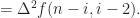
This is exactly $i$ -th finite difference with step $1$ along the $x$ axes, taken at the point $(x,y).$ We have

$\displaystyle f(n-i,i)=f(n-i,i-1)-f(n-i+1,i-1)$

$\displaystyle =\big(f(n-i,i-2)-f(n-i+1,i-2)\big)- \big(f(n-i+1,i-2)-f(n-i+2,i-2) \big)$

$\displaystyle =f(n-i,i-2)-2f(n-i+1,i-2)+f(n-i+2,i-2)$

$\displaystyle =\Delta^2 f(n-i,i-2).$

Proceeding in the same way, it can be obtaned by induction that

$\displaystyle f(n-i,i)=(-1)^i\Delta^i f(n-i,0).\qquad (2).$

Pluging it into $(1)$ yields

$\displaystyle f(0,0)=\sum_{i=0}^n \binom{n}{i} (-1)^{n-i}\Delta^{n-i} f(i,0).\qquad(3)$

In the same way we get

$\displaystyle f(k,0)= \sum_{i=k}^n \binom{n-k}{i-k} (-1)^{n-i}\Delta^{n-i}f(i,0)$

$\displaystyle =\sum_{i=k}^n \frac{i(i-1)\cdots (i-k+1)}{n(n-1)\cdots (n-k+1)} \binom{n}{i}(-1)^{n-i}\Delta^{n-i}f(i,0).$

Clearly

$\displaystyle \left(\frac{i-k+1}{n-k+1}\right)^k \le \frac{i(i-1)\cdots (i-k+1)}{n(n-1)\cdots (n-k+1)} \le \left(\frac{i}{n} \right)^k. \qquad(4)$

Let us denote

$\displaystyle g(k,n):= \sum_{i=k}^n \left(\frac{i}{n} \right)^k\binom{n}{i}(-1)^{n-i} \Delta^{n-i}f(i,0).$

Having in mind $(4)$ it follows

$\displaystyle |f(k,0)-g(k,n)|\le \sum_{i=k}^n \left|\left(\frac{i}{n}\right)^k -\left(\frac{i-k+1}{n-k+1}\right)^k\right|\binom{n}{i}(-1)^{n-i}\Delta^{n-i}f(i,0)$

We used $(-1)^{n-i}\Delta^{n-i}f(i,0)\ge 0,$ which folows from $(2)$ . Therefore,

$\displaystyle |f(k,0)-g(k,n)|\le \max_{i,k\le i\le n}\left|\left(\frac{i}{n}\right)^k -\left(\frac{i-k+1}{n-k+1}\right)^k\right|\cdot \sum_{i=k}^n \binom{n}{i}(-1)^{n-i}\Delta^{n-i}f(i,0)$

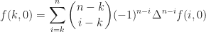
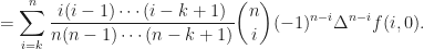
Observe that due to $(3),$ the sum in the right hand side of the above inequality is $1$ . This gives

$\displaystyle |f(k,0)-g(k,n)| \le \max_{i,k\le i\le n}\left|\left(\frac{i}{n}\right)^k -\left(\frac{i-k+1}{n-k+1}\right)^k\right|.$

Note that

$\displaystyle \lim_{n\to\infty} \,\max_{i,k\le i\le n}\left|\left(\frac{i}{n}\right)^k -\left(\frac{i-k+1}{n-k+1}\right)^k\right|=0.$

Thus,

$\displaystyle f(k,0)=\lim_{n\to\infty} \sum_{i=k}^n \left(\frac{i}{n} \right)^k \binom{n}{i} (-1)^{n-i}\Delta^{n-i}f(i,0)$

$\displaystyle = \lim_{n\to\infty} \sum_{i=0}^n \left(\frac{i}{n} \right)^k \binom{n}{i} (-1)^{n-i}\Delta^{n-i}f(i,0) \qquad(5).$

Denote

$\displaystyle A_i:=\binom{n}{i}(-1)^{n-i}\Delta^{n-i}(i,0).$

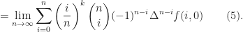
Using the Cauchy-Schwartz inequality, $(3)$ and $(5)$ , we obtain

$\displaystyle f(k,0)^2 = \lim_{n\to\infty} \left( \sum_{i=0}^n \left(\frac{i}{n}\right)^k A_i^{1/2} A_i^{1/2}\right)^2$

$\displaystyle \le \lim_{n\to\infty} \sum_{i=0}^n \left(\frac{i}{n}\right)^{2k}\binom{n}{i}(-1)^{n-i}\Delta^{n-i}f(i,0)\cdot \lim_{n\to\infty}\sum_{i=0}^n \binom{n}{i}(-1)^{n-i}\Delta^{n-i}(i,0).$